Statistics

Mean, standard deviation

# Throw a laplace dice 10000 times. Calculate mean
# and corrected standard deviation of this sample.

use math: sqrt

function mean(a)
   return a.sum()/len(a)
end

function sigma(a,m=null)
   if m is null
      m = mean(a)
   end
   return sqrt(a.sum(|x| (x-m)^2)/(len(a)-1))
end

Stat = table{
   function string()
      return """\
         mean  = {:f4},\n\
         sigma = {:f4}\
      """ % [self.mean, self.sigma]
   end
}

function stat(a)
   m = mean(a)
   return table Stat{mean = m, sigma = sigma(a,m)}
end

s = stat(rng(1..6).list(10000))

print(s)

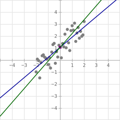
Simple linear regression

LinearRegression = table{
   function string()
      return """\
center = [mx,my]
mx = {mx:f4}
my = {my:f4}
rxy = {rxy:f4}

y(x) = ax*x+bx
ax = {ax:f4}
bx = {bx:f4}

x(y) = ay*y+by
ay = {ay:f4}
by = {by:f4}
""" % record(self)
   end
}

function linear_regression(a)
   vx,vy = list(zip(*a))

   mx = mean(vx)
   my = mean(vy)

   sx = vx.sum(|x| (x-mx)^2)
   sy = vy.sum(|y| (y-my)^2)
   sxy = a.sum(|[x,y]| (x-mx)*(y-my))

   ax = sxy/sx; bx = my-ax*mx
   ay = sxy/sy; by = mx-ay*my

   return table LinearRegression{
      rxy = sxy/sqrt(sx*sy),
      center = [mx,my],
      mx = mx, my = my,
      ax = ax, bx = bx,
      ay = ay, by = by,

      fx = |x| ax*x+bx,
      fy = |y| ay*y+by,
      gx = |y| (y-bx)/ax,
      gy = |x| (x-by)/ay
   }
end

rand = rng()
a = list(-2..2: 0.1).map(|x| [x,x+2*rand()])
r = linear_regression(a)

print(r)

# Let us plot this sample
use plotlib: system

s = system(w=400,h=400,count=5)
s.scatter(a,color=[0.5,0.5,0.5])
s.scatter([r.center],color=[0.5,0,0.5])
s.flush()

s.plot([r.fx,r.gy])

s.idle()

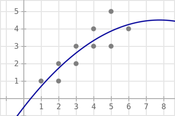
Simple polynomial regression

# The least squares method applied to a polynomial function of
# degree n leads to a linear equation system of n+1 equations.

use math.la: vector, matrix
use math.la.inversion: solve

function regression(points,{degree})
   n = degree
   A = matrix(*(
      list(points.sum(|[x,y]| x^(i+j)) for j in 0..n)
         for i in 0..n))
   w = vector(*(points.sum(|[x,y]| y*x^i) for i in 0..n))
   a = solve(A,w)
   return table{coeff = a, f = |x| (0..n).sum(|k| a[k]*x^k)}
end

use plotlib: system

points = [
   [1,1],[2,1],[2,2],[3,2],[3,3],
   [4,3],[4,4],[5,3],[5,5],[6,4]
]

s = system(w=360,h=240,count=5,align=["left","bottom"])
s.scatter(points,color=[0.5,0.5,0.5])
t = regression(points,degree=2)
s.plot(t.f)
s.idle()

Inverse transform sampling

use math: sqrt,erf
use plotlib: system

# Numerical analysis:
# inversion by bisection method
use math.na: inv


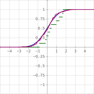
# Inverse transform sampling
function rng_cdf(F)
   rand = rng()
   return || inv(F,rand(),-100,100)
end


# Take a list of random numbers and return the
# cumulative distribution function of this sample.
function cdf(a)
   return |x| a.count(|X| X<=x)/len(a)
end


# CDF: normal distribution
function norm({mu,sigma})
   return |x| 0.5+0.5*erf((x-mu)/sqrt(2*sigma^2))
end


# CDF: standard normal distribution
Phi = norm(mu=0,sigma=1)


X = rng_cdf(Phi)
F1 = cdf(X.list(10))
F2 = cdf(X.list(100))

s = system(w=400,h=400,count=5,scale=[1,0.25])
s.plot([Phi,F1,F2])
s.idle()

Obtaining a CDF from a PMF

use math: pi, exp, sqrt
use math.na: pli, integral


# Optionally, cache the values by
# piecewise linear interpolation.
function cache(f,a,b,d)
   return pli(a,d,list(a..b: d).map(f))
end


erf = |x| 2/sqrt(pi)*integral(0,x,|t| exp(-t^2))
erf = cache(erf,-100,100,0.01)