| ↑ Up |
use math: nan, floor

# By equidistant nodes
# [x0+k*d, y[k]]

function pli(x0,d,y)
   n = len(y)
   return fn|x|
      k = int(floor((x-x0)/d))
      if k<0 or k+1>=n
         return nan
      else
         return y[k]+(y[k+1]-y[k])/d*(x-x0-k*d)
      end
   end
end
# The first derivative of a function f at x
diffh = |h| |f,x| (f(x+h)-f(x-h))/(2*h)
diff = diffh(0.001)


# Differential operator
Dh = |h| |f| |x| (f(x+h)-f(x-h))/(2*h)
D = Dh(0.001)


f = |x| x^2
f1 = D(f)
f2 = (D^2)(f)
function simpson(f,a,b,n)
   h = (b-a)/n
   y = 0
   for i in 0..n-1
      x = a+h*i
      y = y+f(x)+4*f(x+0.5*h)+f(x+h)
   end
   return y*h/6
end
# Gauss-Legendre quadrature nodes,
# GL8 = [x[k],w[k]] for k in 0..7
GL8 = [
   [-0.9602898564975362, 0.1012285362903764],
   [-0.7966664774136267, 0.2223810344533745],
   [-0.5255324099163290, 0.3137066458778874],
   [-0.1834346424956498, 0.3626837833783619],
   [ 0.1834346424956498, 0.3626837833783619],
   [ 0.5255324099163290, 0.3137066458778874],
   [ 0.7966664774136267, 0.2223810344533745],
   [ 0.9602898564975362, 0.1012285362903764]
]

function gauss(f,a,b,n)
   h = (b-a)/n
   p = 0.5*h
   s = 0
   for j in 0..n-1
      q = p+a+j*h
      sj = 0
      for t in GL8
         sj += t[1]*f(p*t[0]+q)
      end
      s += p*sj
   end
   return s
end
# piecewise linear interpolation
use math.na: pli


# y'(x) = f(x,y(x))
# h: step size
# N: number of steps
function euler(f,{x0,y0,h,N})
   x = x0; y = y0
   a = [y]
   for k in 1..N
      y = y+h*f(x,y)
      x = x0+k*h
      a.push(y)
   end
   return pli(x0,h,a)
end


# y^(m)(x) = f(x,y)
# y = [y(x),y'(x),...,y^(m-1)(x)]
function euler_any_order(f,{x0,y0,h,N})
   x = x0; y = copy(y0)
   m = len(y)
   a = [y[0]]
   for k in 1..N
      hf = h*f(x,y)
      for i in 0..m-2
         y[i] = y[i]+h*y[i+1]
      end
      y[m-1] = y[m-1]+hf
      x = x0+k*h
      a.push(y[0])
   end
   return pli(x0,h,a)
end


exp = euler(|x,y| y,{
   x0=0, y0=1, h=0.01, N=1000
})

sin = euler_any_order(|x,y| -y[0],{
   x0=0, y0=[0,1], h=0.01, N=1000
})
use plotlib: system
use math.ode: runge_kutta
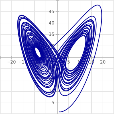
# Lorenz attractor
x,y,z = runge_kutta({
f = |t,[x,y,z]| [
10*(y-x),
x*(28-z)-y,
x*y-8/3*z
],
t0=0, y0 = [1,1,1],
w=40, unilateral = true
})
s = system(w=400,h=400,scale=5,origin=[0,25],count=5)
s.vplot(|t| [x(t),z(t)], {t0=0, t1=40, n=4000})
s.idle()
use plotlib: system
use math.la: vector
use math.ode: runge_kutta

# Motion around a fixed center of mass,
# by Newton's law of gravitation:
#   x''(t) = -GM*x/|x|^3.

G=1; M=1

x,v = runge_kutta({
   f = |t,[x,v]| [v, -G*M*x/abs(x)^3],
   y0 = [vector(4,3),vector(0,0.28)],
   t0 = 0, h=0.01, w=100,
   unilateral = true
})

s = system(dark=true,w=400,h=400,count=5)
s.scatter(x[0..34])
s.idle()

# n-body simulation,
# by Newton's law of gravitation:
#   x[i]''(t) = G*sum(k!=i) m[k]*(x[k]-x[i])/|x[k]-x[i]|^3.

use plotlib: system
use math.la: vector
use math.ode: runge_kutta

function nbody({G,m})
   n = len(m)
   vindex = vector(*list(0..n-1))
   return |x| vindex.map(|i| G*(0..n-1).sum(|k|
      vector(0,0) if k==i else
      m[k]*(x[k]-x[i])/abs(x[k]-x[i])^3))
end

m,x0,v0 = list(zip(
   # Star
   [1, vector(0,0), vector(0,0)],

   # Planet
   [0.01, vector(4,0), vector(0,0.4)],

   # Moon
   [0.0001, vector(4.1,0), vector(0,0.2)]
))

x0 = vector(*x0)
v0 = vector(*v0)
g = nbody(G=1,m=m)

x,v = runge_kutta({
   f = |t,[x,v]| [v,g(x)],
   y0 = [x0,v0],
   t0 = 0, h=0.01, w=100,
   unilateral = true
})

s = system(dark=true,w=720,h=480,count=5)

for t in 0..31:0.1
   xt = x(t)

   s.rgb(0.8,0.7,0)
   s.scatter([xt[0]], radius=0.5)

   s.rgb(0.6,0.6,0.8)
   s.scatter([xt[1]], radius=0.1)

   s.rgb(0,0.6,0.6)
   s.scatter([xt[2]], radius=0.02)
end

s.idle()

use math: pi, exp

# Fast Fourier transform of a.
# Note: len(a) is a power of two.

function fft(a)
   if len(a)<=1
      return copy(a)
   else
      even = fft(a[0..:2]); odd = fft(a[1..:2])
      N = len(a); L = list(0..N//2-1)
      T = L.map(|k| exp(-2i*pi*k/N)*odd[k])
      return (L.map(|k| even[k]+T[k])+
              L.map(|k| even[k]-T[k]))
   end
end
What follows is an approximation of the complex Riemann zeta function ζ(s) by an application of the Euler-MacLaurin formula, which yields:
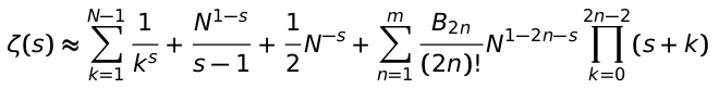
At next this calculation will be implemented without further ado. Finally the functional equation of the zeta function (a.k.a. reflection formula) is used for Re(s)<0.
use math: pi, sin, gamma
use math.sf: B
use cmath: re

function new_zeta({N,m})
   function Euler_MacLaurin_term(s,N,m)
      return (1..m).sum(|n| B(2*n)/gamma(2*n+1)
         *N^(1-2*n-s)*(0..2*n-2).prod(|k| (s+k)))
   end
   function zeta_Euler_MacLaurin(s,N,m)
      return ((1..N-1).sum(|k| 1/k^s)+N^(1-s)/(s-1)
         +0.5*N^(-s)+Euler_MacLaurin_term(s,N,m))
   end
   return fn zeta|s|
      if re(s)<0
         return (2^s*pi^(s-1)*sin(pi*s/2)
            *gamma(1-s)*zeta_Euler_MacLaurin(1-s,N,m))
      else
         return zeta_Euler_MacLaurin(s,N,m)
      end
   end
end

zeta = new_zeta(N=12,m=6)